Filling SpatialPolygons with an image

Plotting country outlines is really easy in R, but making those plots a bit more fancy can be frustrating. I thought it would be nice to fill the country outlines with an image rather than with a solid colour. How hard could it be? After some googling it appears that there is very little documentation on this topic. The only document that I found was by Paul Murrel (2011). He plots a black filled country shape first and then captures the rasterized shape using the grid.cap function from the grid package. This captured raster is then used as a mask on the image that needs to be plotted in the shape of a country.

I'm having difficulties with this approach for two reasons: one, I can't seem to get grid.cap working as it should; two, I don't like having to plot the shape of a country first in order to create a mask. The first matter is probably my own wrongdoing, but all the grid.cap function returns me is a matrix of white pixels. I grew tired of figuring out what I was doing wrong. For the second aspect, I think a more direct approach should be possible by using the ‘over’ function from the sp package.

So these are the steps that I took to tackle the problem:

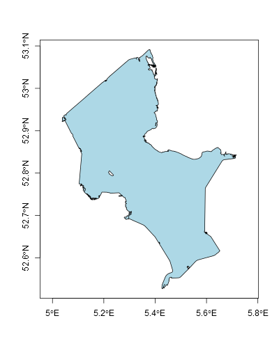
1. Download the country shape
2. Download a suitable png image
3. Georeference the image, such that it matches the location of the country
4. Use the ‘over’ function to determine which pixels are inside the country shape
5. Plot the pixels of the image that are inside the country and plot the outline

In this post I will show you how to create the image shown below, where each country is filled with an image of their respective flag. Below I will explain in a bit more detail how this image was created, following the steps listed above. I've also provided the script used to create the image below, where each of the steps are also clearly marked.

The country shapes for step 1 are downloaded from GADM using the getData function from the raster package. Of course you can use any SpatialPolygons object from any other source.

The country flag png images are downloaded from wikipedia (step 2). So this example shows how to download png image and turn it into a usable format. If you like, you can use any image format like jpg or tif, but that will require some modification of the code presented here.

To understand the next step (3), I'm using georeferencing and I may need to explain what that means. Basically, this is telling where and how the image should be positioned in the coordinate reference system (CRS) of the SpatialPolygons objects (the country outlines). In this step I'm instructing the system to stretch the image to the bounding box of the respective country. This also means that the aspect ratio of the original image is probably messed up. If you would like to keep the original aspect ratio, you need to modify this step. The image was downloaded as an array with the red, green and blue component in separate dimensions. With the brick function from the raster package this array is turned into a correctly georeferenced brick object.

Now that we have properly positioned the image, we need to determine which pixels are located inside the country outlines (step 4). For this purpose, we use the ‘over’ function from the sp package. This function will not accept a raster brick object as input. The raster brick object is therefore cast into a SpatialGrid format. The function will return a dataframe with the country shape element that matches with a specific grid cell. From this information it can be derived whether the pixel is situated inside or outside the country outline. The pixel values for those situated outside the country outlines are set to NA. Note that this can be a time-consuming step. Especially when the resolution of your image is high, and/or the country outline is complex (i.e., contains details, a lot of islands and/or holes), so either be patient. Alternatively, you can speed up the process by either lowering the resolution of your image (hint: focal) or simplifying the country outline (hint: gSimplify).

All there is left to do is to plot the image and the outline (step 5). I use the plotRGB function from the raster package to plot the image. Don't forget to set the ‘bgalpha’ argument to 0, to ensure that NA values are plotted as transparent pixels. Otherwise, it will plot white pixels over anything that has previously been plotted.

I've wrapped four of the five steps in a function, such that I could easily repeat these steps for different countries. Hopefully this post will help you to create your own cool graphics in R. Good luck, and please let me know in the comments if any of the steps are not clear...

Segmenting SpatialPolygons

Both SpatialPolygons and SpatialPolygons consist of list of Polygons. Each of these Polygons in turn consist of vertices, i.e., the points where the edges of the polygon meet. When you transform a SpatialPolygons(DataFrame) to a different projection (e.g., from long-lat coordinates to UTM) with the spTransform-function, actually only the vertices are transformed (and not the lines connecting them). This means that also in the new projection straight lines are drawn between the vertices, whereas in reality they should be curved (due to the quasi-spherical shape of our world). For most shapes this isn't much of an issue. But when your shape covers a large area, you could run into serious problems.

This problem can be solved by adding more vertices to the polygons. In other words, add new vertices by interpolating between the existing vertices. If you do this before re-projecting, the new projection will be a lot more accurate. I tried to find an existing package in R that would do this, but I could not find any (please leave a comment if you did find an alternative). Therefore, I've written a small function to take care of this myself, which I will demonstrate in this post.

The source code of this function and the accompanying example is given below. This code is also used to produced the graphical illustration below. Note how the red line crosses the islands Northeast of Scotland in the original projection. Compare this with the new projection of the red lines with and without segmentation. Also note that the red lines in the new projection are straight when we don't apply segmentation, and they are curved (as they are supposed to be) when we do apply segmentation.

The segmentation is achieved relatively simple by looping all the lists of Polygons with the lapply function and then looping each line segment with the apply function (see R script below). The new vertices are derived via linear interpolation using the approx function. You could go for something more fancy like spline interpolation, but linear will do just fine in this example. As I've implemented all this in the function named ‘SPSegmentation’, you can simply call it on any SpatialPolygons or SpatialPolygonsDataFrame object you would like. With some modifications, you could also use this function of SpatialLines and SpatialLinesDataFrame objects.

In case you want to achieve the opposite (i.e., reduce the number of vertices in a SpatialPolygons(DataFrame)), you can use the gSimplify function from the rgeos package. This uses a Ramer–Douglas–Peucker algorithm to simplify the shape, which could save you some computing time, but your shape will also become less detailed as a result.

Openstreetmap relation, please be a SpatialPolygons object

The sp package is the package when it comes to handling spatial data in R. Getting to know how this package work can take some time, but it's well worth it. It can be a pain to import spatial data from for instance www.opentreetmap.org.

The other day for instance, I required an outline of Lake IJssel. How hard could it be to get that from openstreetmap? Well, getting the data is not all that hard, but converting it into something workable really got me pulling my hair out. In order to save future frustrations, I decided to share my solution with you.

The first step is to get the relation id number from openstreetmap. This can be easily obtained by searching the website for ‘Lake IJssel’. After clicking the first hit that represents a water body, you will find the relation id.

The second step is to download the data in R using this relation id. This can be done with the get_osm function of the osmar package. This data can be converted into a SpatialLines object using the as_sp function from the osmar package. However, I don't want a SpatialLines object; I want it to be a SpatialPolygons object. And that is the tricky bit, because there is no package available (that I know of) that can do this directly.

So this is the trick that I applied. First you need to join the lines in the SpatialLines object, using the gLineMerge function from the rgeos package (it took me a while to figure this one out!). Then convert it into a PolySet using the SpatialLines2PolySet function from the maptools package. Only then can it be converted into a SpatialPolygons object using the PolySet2SpatialPolygons function from the maptools package. If anyone knows of an easier way, pleas let me know in the comments.

So, there you have it. A SpatialPolygons object of Lake IJssel, that is actually useful for my purpose. The code below will do what I've described in this post; feel free to try it yourself! Note that it may not work on all openstreetmap data...